PVBM Tutorial

If you are using colab, install the pvbm library by uncommenting the following cell

[1]:

#pip install pvbm --upgrade``

Import the libraries

[2]:

%load_ext autoreload
%autoreload 2

[3]:

from PIL import Image
import numpy as np
import matplotlib.pyplot as plt
from skimage.morphology import skeletonize,square,dilation
import os
import pathlib
import sys
from matplotlib.colors import ListedColormap

sys.setrecursionlimit(100000)

Download the PVBM datasets

[4]:

path_to_save_datasets = "../PVBM_datasets"

[5]:

from PVBM.Datasets import PVBMDataDownloader
dataset_downloader = PVBMDataDownloader()
dataset_downloader.download_dataset(name="Crop_HRF", save_folder_path=path_to_save_datasets)
dataset_downloader.download_dataset(name="INSPIRE", save_folder_path=path_to_save_datasets)
dataset_downloader.download_dataset(name="UNAF", save_folder_path=path_to_save_datasets)
print("Images downloaded successfully")

Downloading...
From (original): https://drive.google.com/uc?id=1QcozuK5yDyXbBkHqkbM5bxEkTGzkPDl3
From (redirected): https://drive.google.com/uc?id=1QcozuK5yDyXbBkHqkbM5bxEkTGzkPDl3&confirm=t&uuid=a2d7d6ed-dbaf-4d83-b4d2-2b8457e2023d
To: /Users/jonathanfhima/Desktop/PVBMRelated/PVBM/Crop_HRF.zip
100%|█████████████████████████████████████████████████████████████████████████████████████████████████████████████████████████████| 42.0M/42.0M [00:01<00:00, 28.0MB/s]

Dataset downloaded and saved to Crop_HRF.zip
Files extracted to ../PVBM_datasets
Deleted the zip file: Crop_HRF.zip

Downloading...
From (original): https://drive.google.com/uc?id=18TcmkuN_eZgM2Ph5XiX8x7_ejtKhA3qb
From (redirected): https://drive.google.com/uc?id=18TcmkuN_eZgM2Ph5XiX8x7_ejtKhA3qb&confirm=t&uuid=673cf335-4396-45cc-ba47-7b4c13e3f14c
To: /Users/jonathanfhima/Desktop/PVBMRelated/PVBM/INSPIRE.zip
100%|█████████████████████████████████████████████████████████████████████████████████████████████████████████████████████████████| 29.6M/29.6M [00:01<00:00, 27.8MB/s]

Dataset downloaded and saved to INSPIRE.zip
Files extracted to ../PVBM_datasets
Deleted the zip file: INSPIRE.zip

Downloading...
From: https://drive.google.com/uc?id=1IM5qUEARNp2RFpzKmILbdgasjLuJEIcX
To: /Users/jonathanfhima/Desktop/PVBMRelated/PVBM/UNAF.zip
100%|█████████████████████████████████████████████████████████████████████████████████████████████████████████████████████████████| 19.7M/19.7M [00:00<00:00, 20.7MB/s]

Dataset downloaded and saved to UNAF.zip
Files extracted to ../PVBM_datasets
Deleted the zip file: UNAF.zip
Images downloaded successfully

[6]:

list(pathlib.Path(path_to_save_datasets).glob("*/*"))

[6]:

[PosixPath('../PVBM_datasets/Paraguay_crop/artery'),
 PosixPath('../PVBM_datasets/Paraguay_crop/veins'),
 PosixPath('../PVBM_datasets/Paraguay_crop/images'),
 PosixPath('../PVBM_datasets/Paraguay_crop/unknown'),
 PosixPath('../PVBM_datasets/INSPIRE/artery'),
 PosixPath('../PVBM_datasets/INSPIRE/veins'),
 PosixPath('../PVBM_datasets/INSPIRE/images'),
 PosixPath('../PVBM_datasets/INSPIRE/labels'),
 PosixPath('../PVBM_datasets/__MACOSX/._CropHRF'),
 PosixPath('../PVBM_datasets/__MACOSX/CropHRF'),
 PosixPath('../PVBM_datasets/CropHRF/artery'),
 PosixPath('../PVBM_datasets/CropHRF/veins'),
 PosixPath('../PVBM_datasets/CropHRF/images'),
 PosixPath('../PVBM_datasets/CropHRF/unknown')]

Load an image

[7]:

segmentation_path = list(pathlib.Path(path_to_save_datasets).glob("INSPIRE/artery/*"))[0]
segmentation_path

[7]:

PosixPath('../PVBM_datasets/INSPIRE/artery/image8.png')

[8]:

segmentation = Image.open(segmentation_path) #Open the segmentation

[9]:

plt.imshow(segmentation,cmap = "gray") #Display the segmentation
plt.title("Segmentation")
plt.axis('off')
plt.show()

[10]:

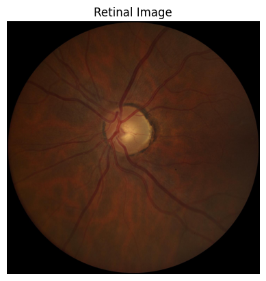
image_path = str(segmentation_path).replace("artery","images").replace("veins", "images")
image = Image.open(image_path)
plt.imshow(image) #Display the segmentation
plt.title("Retinal Image")
plt.axis('off')
plt.show()

[11]:

segmentation = np.array(segmentation)/255 #Convert the segmentation to a numpy array with value 0 and 1
skeleton = skeletonize(segmentation)*1 #Compute the skeleton of the segmentation

[12]:

plt.imshow(skeleton,cmap = 'gray')
plt.title("Segmentation skeleton")
plt.axis('off')
plt.show()

Extract the optic disc

[13]:

from PVBM.DiscSegmenter import DiscSegmenter
segmenter = DiscSegmenter()

Model path: /Users/jonathanfhima/Desktop/PVBMRelated/PVBM/PVBM/lunetv2_odc.onnx
Model already exists, skipping download.

[14]:

optic_disc = segmenter.segment(image_path=str(segmentation_path).replace("artery","images").replace("veins", "images"))

[15]:

plt.imshow(optic_disc)
plt.title("optic disc")
plt.axis('off')
plt.show()
plt.imshow(image)
plt.title("Retinal Image")
plt.axis('off')
plt.show()

[16]:

#Compute the center and radius of the optic disc, as well as the Region of Interest (ROI) on which the Geometrical VBMs will be computed
#And the zones ABC on which the Central Retinal Equivalent will be computed
center, radius, roi, zones_ABC = segmenter.post_processing(segmentation=optic_disc, max_roi_size=600)

[17]:

center

[17]:

(682, 620)

[18]:

radius

[18]:

[19]:

plt.imshow(image)
plt.imshow(roi, alpha = 0.3)
plt.title("ROI used to compute the geometrical VBMs")
plt.axis('off')
plt.show()

[20]:

plt.imshow(image)
plt.imshow(zones_ABC/255, alpha = 0.5)
plt.title("Zones A, B and C")
plt.axis('off')
plt.show()

Compute the geometrical VBMs

[21]:

from PVBM.GeometryAnalysis import GeometricalVBMs #Import the geometry analysis module
geometricalVBMs = GeometricalVBMs() #Instanciate a geometrical VBM object

[22]:

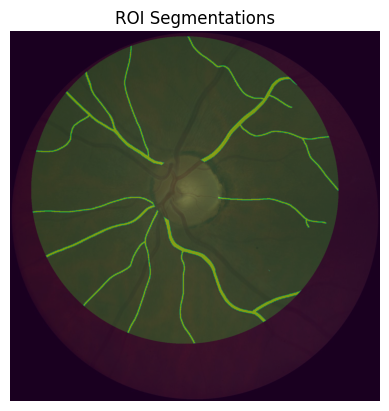
segmentation_roi, skeleton_roi = geometricalVBMs.apply_roi(
    segmentation=segmentation,
    skeleton=skeleton,
    zones_ABC=zones_ABC,
    roi=roi
)

[23]:

plt.imshow(image)
plt.imshow(segmentation_roi, alpha = 0.5)
plt.imshow(roi, alpha = 0.2)
plt.title("ROI Segmentations") #Segmentation within the ROI that will be used for the geometrical VBMs
plt.axis('off')
plt.show()

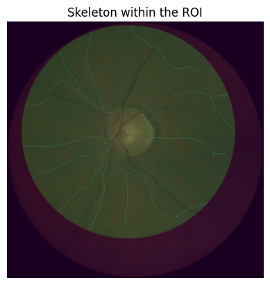
[24]:

plt.imshow(image)
plt.imshow(skeleton_roi, alpha = 0.5)
plt.imshow(roi, alpha = 0.2)
plt.title("Skeleton within the ROI") #that will be used for the geometrical VBMs
plt.axis('off')
plt.show()

[25]:

vbms, visual = geometricalVBMs.compute_geomVBMs(
    blood_vessel=segmentation_roi,
    skeleton=skeleton_roi,
    xc=center[0],
    yc=center[1],
    radius=radius
)

[26]:

area, TI, medTor, ovlen, medianba, startp, endp, interp = vbms
area, TI, medTor, ovlen, medianba, startp, endp, interp
print(f"\n Area : {area} \n Tortuosity Index: {TI} \n Median Tortuosity: {medTor}\n Overall Length {ovlen} \n Median Branching angles {medianba}\n Number of Start/End/Intersection points {startp}/ {endp} / {interp}")


 Area : 52340.0
 Tortuosity Index: 1.094966815867056
 Median Tortuosity: 1.0822196059435547
 Overall Length 6734.379577000198
 Median Branching angles 77.68055474336339
 Number of Start/End/Intersection points 7/ 18.0 / 11.0

[27]:

endpoints, interpoints, startpoints, angles_dico, topology_dico = visual

Plot the branching angles

[28]:

import numpy as np
import matplotlib.pyplot as plt
from skimage.draw import line_aa
from scipy.ndimage import binary_dilation


def display_angles(angles_dico, img):
    for key, value in angles_dico.items():
        b = key
        if len(value) == 2:
            a, c = value
            if all(x is not None for x in (a, b, c)):
                ba = np.array(a) - np.array(b)
                bc = np.array(c) - np.array(b)
                cosine_angle = np.dot(ba, bc) / (np.linalg.norm(ba) * np.linalg.norm(bc))
                angle = np.arccos(cosine_angle)
                rr, cc, val = line_aa(b[0], b[1], a[0], a[1])
                img[rr, cc] = val * 255
                rr, cc, val = line_aa(b[0], b[1], c[0], c[1])
                img[rr, cc] = val * 255
                plt.text(b[1], b[0], f"{np.degrees(angle):.1f}", color='red', fontsize=8)
        elif len(value) == 3:
            a, c, d = value
            if all(x is not None for x in (a, b, c, d)):
                # First angle (a-b-c)
                ba = np.array(a) - np.array(b)
                bc = np.array(c) - np.array(b)
                cosine_angle_ac = np.dot(ba, bc) / (np.linalg.norm(ba) * np.linalg.norm(bc))
                angle_ac = np.arccos(cosine_angle_ac)
                rr, cc, val = line_aa(b[0], b[1], a[0], a[1])
                img[rr, cc] = val * 255
                rr, cc, val = line_aa(b[0], b[1], c[0], c[1])
                img[rr, cc] = val * 255
                plt.text(b[1], b[0], f"{np.degrees(angle_ac):.1f}", color='red', fontsize=8)

                # Second angle (c-b-d)
                bc = np.array(c) - np.array(b)
                bd = np.array(d) - np.array(b)
                cosine_angle_cd = np.dot(bc, bd) / (np.linalg.norm(bc) * np.linalg.norm(bd))
                angle_cd = np.arccos(cosine_angle_cd)
                rr, cc, val = line_aa(b[0], b[1], c[0], c[1])
                img[rr, cc] = val * 255
                rr, cc, val = line_aa(b[0], b[1], d[0], d[1])
                img[rr, cc] = val * 255
                plt.text(b[1], b[0] + 10, f"{np.degrees(angle_cd):.1f}", color='red', fontsize=8)

img = np.zeros_like(segmentation)

display_angles(angles_dico, img)

# Dilate the image
img_dilated = binary_dilation(img, structure=np.ones((8,8))) * 255

plt.imshow(image)
plt.imshow(segmentation_roi, alpha = 0.5)
plt.imshow(roi, alpha = 0.2)
plt.imshow(img_dilated, cmap='gray', alpha = 0.3)
plt.axis('off')
plt.show()

Plot the particular points

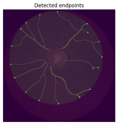
[29]:

plt.imshow(image)
plt.imshow(segmentation_roi, alpha = 0.5)
plt.imshow(roi, alpha = 0.2)
plt.imshow(segmentation/50+dilation(endpoints, square(15)), alpha = 0.5)
plt.title("Detected endpoints")
plt.axis('off')
plt.show()

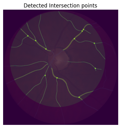
[30]:

plt.imshow(image)
plt.imshow(segmentation_roi, alpha = 0.5)
plt.imshow(roi, alpha = 0.2)
plt.imshow(segmentation/20+dilation(interpoints, square(15)), alpha = 0.5)
plt.title("Detected Intersection points")
plt.axis('off')
plt.show()

[31]:

plt.imshow(image)
plt.imshow(segmentation_roi, alpha = 0.5)
plt.imshow(roi, alpha = 0.2)
plt.imshow(segmentation/20+dilation(startpoints, square(15)), alpha = 0.5)
plt.title("Detected startpoints")
plt.axis('off')
plt.show()

Plot the linear interpolation of the particular points

[32]:

from skimage.draw import line_aa
import matplotlib.pyplot as plt
import numpy as np
from scipy.ndimage import binary_dilation

img = np.zeros_like(segmentation)

for key, value in topology_dico.items():
        rr, cc, val = line_aa(key[0], key[1], key[2], key[3])
        img[rr, cc] = val * 255
        plt.text(key[3], key[2], f"{value[0]/value[1]:.3f}", color='red', fontsize=8)

# Dilate the image
img_dilated = binary_dilation(img, structure=np.ones((8,8))) * 255

plt.imshow(image)
plt.imshow(segmentation_roi, alpha = 0.5)
plt.imshow(roi, alpha = 0.2)
plt.imshow(img_dilated, cmap='gray', alpha = 0.3)
plt.axis('off')
plt.show()

Fractal Analysis

[33]:

from PVBM.FractalAnalysis import MultifractalVBMs
fractalVBMs = MultifractalVBMs(n_rotations = 25,optimize = True, min_proba = 0.0001, maxproba = 0.9999)

[34]:

D0,D1,D2,SL = fractalVBMs.compute_multifractals(segmentation_roi.copy())

[35]:

print("The fractal biomarkers are D0: {}, D1: {}, D2: {}, SL: {}".format(D0,D1,D2,SL))

The fractal biomarkers are D0: 1.3344921958711857, D1: 1.2982229835136063, D2: 1.2798524605762445, SL: 0.9573680985889439

Central Retinal Equivalent Analysis

[36]:

from PVBM.CentralRetinalAnalysis import CREVBMs
creVBMs = CREVBMs()

[37]:

segmentation_roi, skeleton_roi = creVBMs.apply_roi(
    segmentation=segmentation,
    skeleton=skeleton,
    zones_ABC=zones_ABC
)

[38]:

plt.imshow(segmentation_roi)
plt.imshow(zones_ABC/255, alpha = 0.5)
plt.axis('off')
plt.title("ROI for CRE biomarkers")
plt.show()

[39]:

#This allows to generate the CRE visualisation but require a lot of RAM
#If you are only interested about the VBMs values then set it to False
plot = True

[40]:

out = creVBMs.compute_central_retinal_equivalents(
    blood_vessel=segmentation_roi.copy(),
    skeleton=skeleton_roi.copy(),
    xc=center[0],
    yc=center[1],
    radius=radius,
    artery = True,
    Toplot = plot
)

/opt/homebrew/lib/python3.11/site-packages/numpy/core/fromnumeric.py:3504: RuntimeWarning: Mean of empty slice.
  return _methods._mean(a, axis=axis, dtype=dtype,
/opt/homebrew/lib/python3.11/site-packages/numpy/core/_methods.py:129: RuntimeWarning: invalid value encountered in scalar divide
  ret = ret.dtype.type(ret / rcount)

[41]:

if out == -1:
    raise ValueError("The CRE computation failed")
else:
    output, visualisation = out
    print(output)

{'craek': 17.597833412365436, 'craeh': 19.17509597260818}

[42]:

if plot:
    # Load all the logs to build the cre visualisation
    measurements = [item['plot'] for item in visualisation]
    # Compute the aggregated visualisation
    measurements = np.maximum.reduce(measurements)

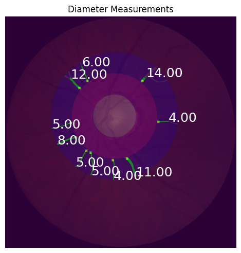
[43]:

if plot:

    # Create a new figure
    plt.imshow(image)
    plt.imshow(segmentation_roi, alpha = 0.3)
    plt.imshow(zones_ABC/255, alpha = 0.5)
    plt.imshow(measurements)


    startpoints_cre = np.zeros((segmentation_roi.shape[0], segmentation_roi.shape[1]))

    # Annotate the image with 'Mean diameter' from each dictionary
    for item in visualisation:

        startpoints_cre[item["start"]] = 1
        # Get the 'end' location and 'Mean diameter'
        end_location = item['end']  # Assuming 'end' is a tuple (x, y)
        mean_diameter = "{:.2f}".format(item['Median diameter'])

        # Annotate the image
        plt.annotate(mean_diameter,
                     (end_location[1], end_location[0]),
                     color='white',
                     fontsize=18)

    # Display the combined image
    plt.imshow(dilation(startpoints_cre, square(15)), alpha = 0.5)

    plt.axis('off')
    plt.tight_layout()
    plt.title("Diameter Measurements")
    plt.show()

[ ]: